An Introduction to Gradient Descent
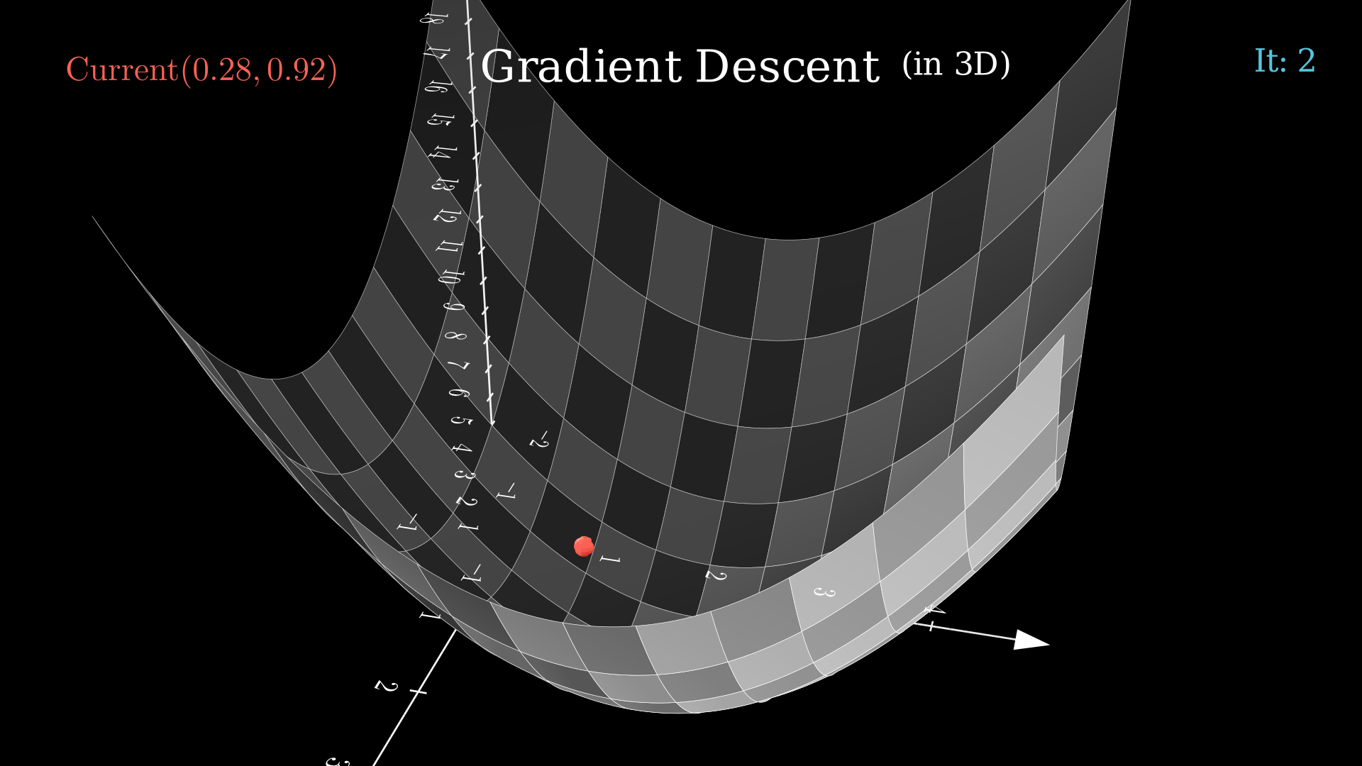
Table of Contents
Introduction
Gradient Descent (GD) is a fundamental optimization algorithm used to find the minimum of a function. In machine learning, it's often applied to optimize a loss function by iteratively moving toward the direction of steepest descent. GD is the secret sauce behind the success of many machine learning algorithms and neural networks.
GD works by taking small steps in the direction of the negative gradient of the function. Mathematically, it can be expressed as:
Let's start from the basics to better understand what the various terms in the equation mean.
Preliminary
One does not need much academic knowledge to understand the GD algorithm. This section introduces some basic concepts that will help us understand the algorithm better.
Function
A function is just a mapping with a condition that each input must be mapped to only one output. We can treat a function like a machine that, given a specific input(s), returns specific output(s). These inputs and outputs can be anything from natural numbers to vectors of complex numbers. Formally, a function from a set to a set assigns to each element of exactly one element of . The set is called the domain of the function and the set is called the codomain of the function.1
For example, we can define a function that always returns the square of what was passed to it. Assuming that we pass a real number, the function is written as:
with and . Note that the output is always a positive number and hence the codomain of the function is the set of positive real numbers.
Derivative
Derivative is a measure of how a function changes as its input changes. It gives the rate of change of the function at a particular point. From a geometric point of view, the derivative of a function at a point is the slope of the tangent line to the function at that point. For a function of more than one variable, we are more interested in what is known as partial derivatives. The partial derivative of a multivariate function with respect to a variable is the derivative of the function where all the variables are assumed to be constant.
Let’s talk about some notations. The derivative of a univariate function is denoted as or . For a multivariate function , the partial derivative of the function with one of its variables, say can be written as or .
Gradient
The gradient is just a special case of derivative. It is the slope of a curve at a given point in a specified direction. For a univariate function, the gradient is equal to the function's derivative at that point. For multivariate function, it is defined as:
Here, is the point of interest.
Requirements for GD
For a GD algorithm to work, the function needs to satisfy two key requirements. The function should be:
- differentiable, and
- convex
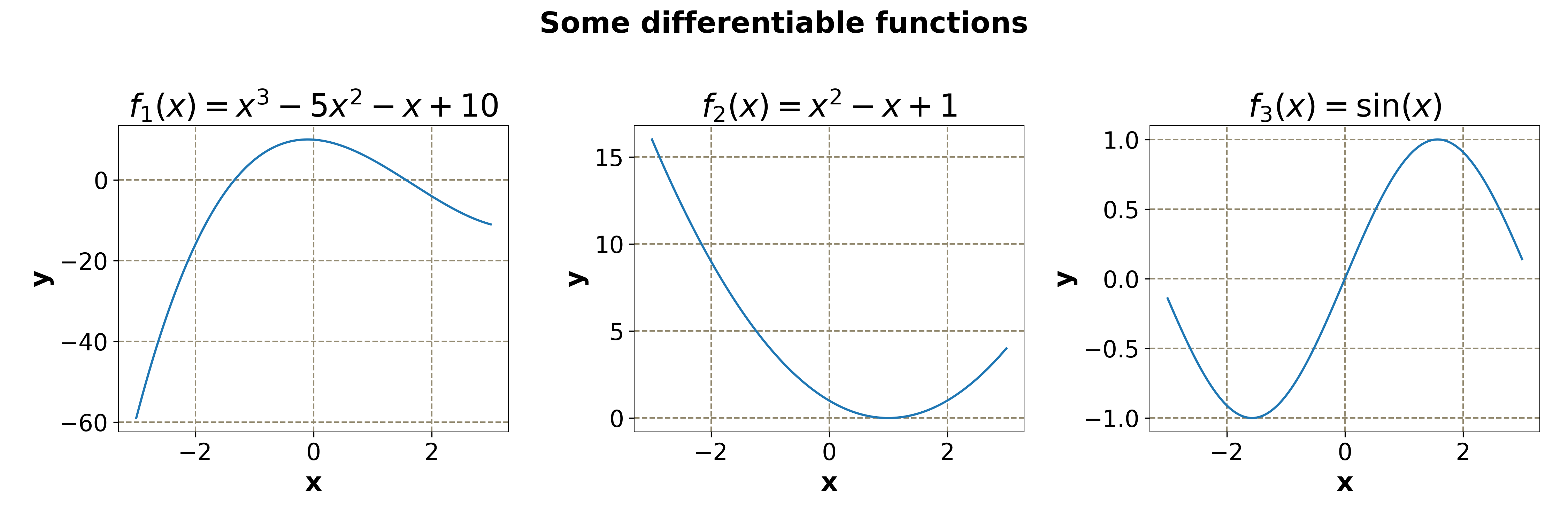
Differentiability
A function is differentiable if it has a derivative at all points of its domain. The following are some examples of functions that are differentiable.
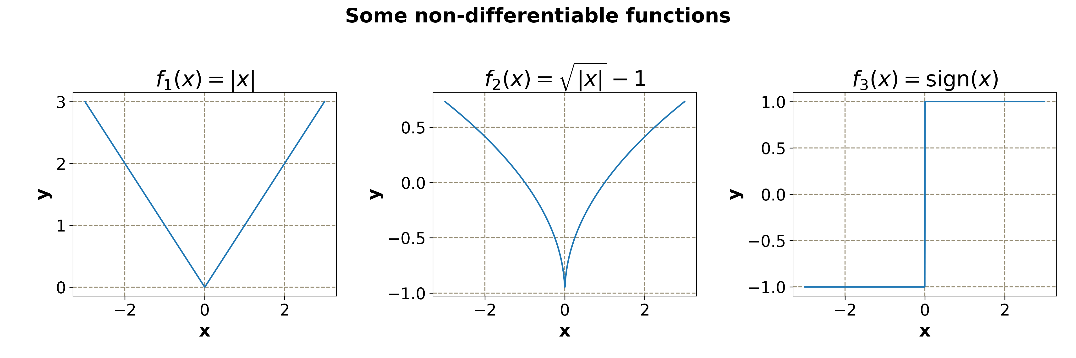
Not all functions are differentiable. Here are some examples of non-differentiable functions.
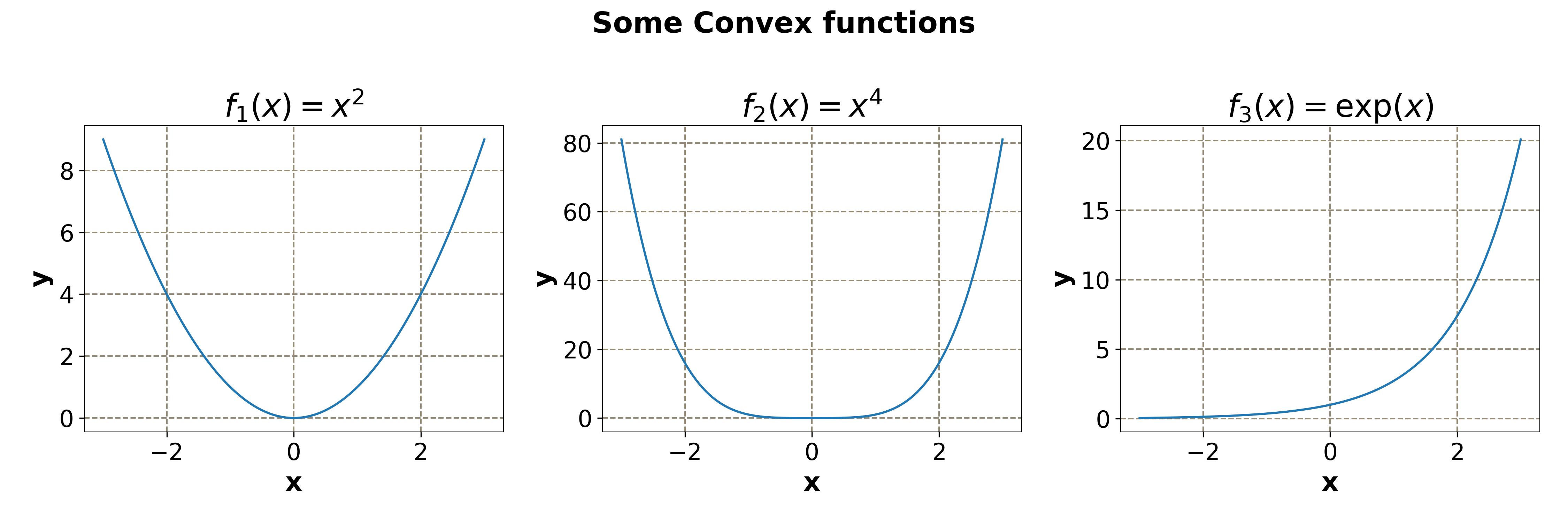
Convexity
Geometrically speaking, for a function of a single variable to be convex, the line connecting any two points on the curve must be on or above the curve. The same is also true of a convex function of more than one variable, if we replace the line to a high-dimensional representation of a line (for example, in 3D, it will be a place) and the two points to a set of points.
Mathematically, a function is said to be convex, if for and in domain of , the following condition hold2:
Some examples are:
For a convex function, the line between a fixed point and any other point on the curve always remains above the curve. The result will remain unchanged even if one changes the fixed point.
A straightforward way to check if a univariate function is convex is to calculate the second derivative and check if its value is always bigger than 0.
Of course, not all functions are convex.
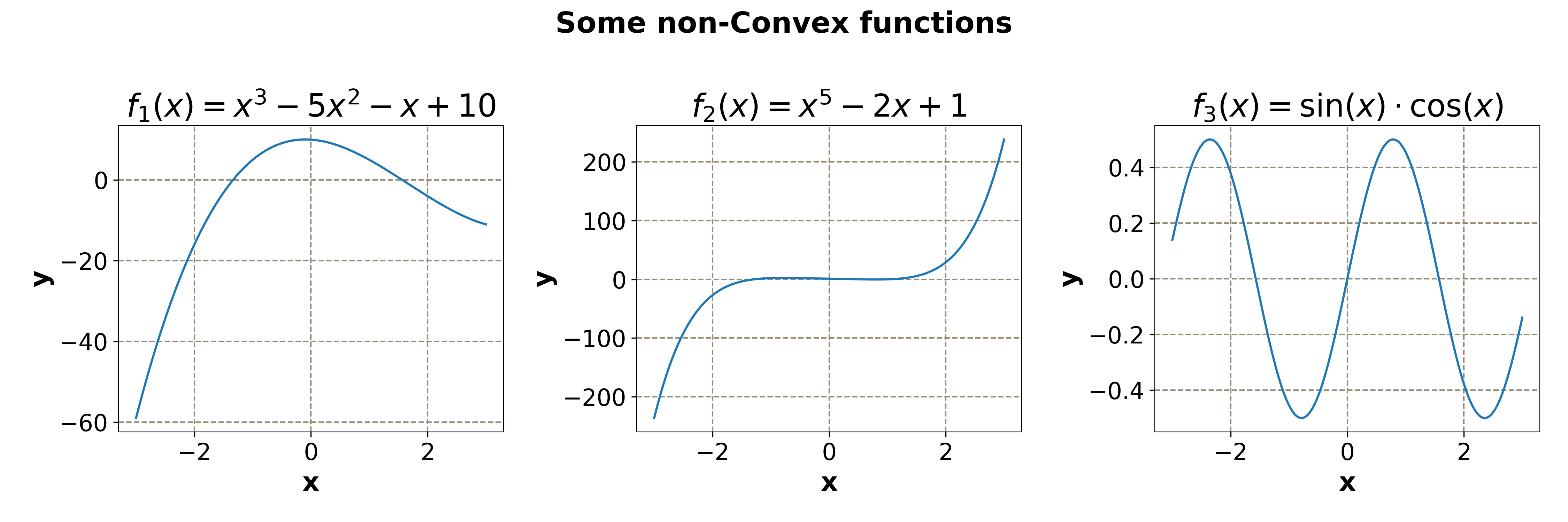
There are some functions that are convex in some domains and non-convex (concave) in other domains. These are called quasi-convex functions. GD algorithm works on these types of functions too. However, these functions contain some points, called saddle points, where the convexity of the function changes, and the GD can get stuck on these points (as we will see later). One example of such a function is . By taking the second derivative, one can verify that this function has a saddle point at and it is:
- convex for
- concave for
- convex again for
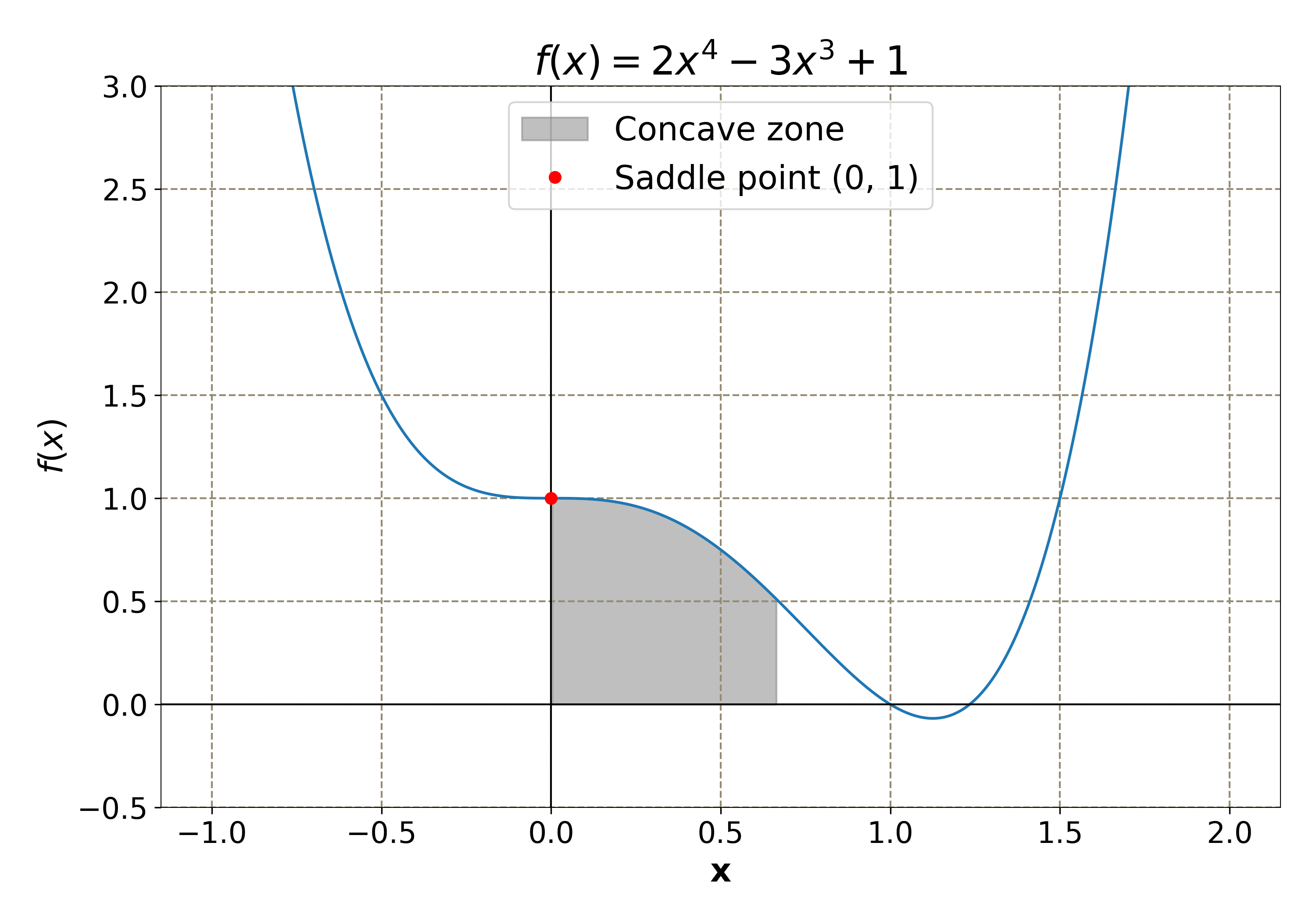
The quasi-convex function . The saddle point is shown as a red dot. The region where the function is concave is shaded.
The animation shows why the function is not convex. Note that the line connecting the two points does not always remain above the curve. The line color turns red when it lies below the curve (which happens between and ). As the second point moves from right to left, the text indicating whether the point lies in the convex or non-convex zone also changes.
The Algorithm
Now that we are familiar with the terms used in the GD equation, we are ready to understand the algorithm. Let be a function with parameters that we need to optimize. Note that can be a scalar or a vector. For this, the GD algorithm is:
- Initialize the parameters with some random values, say .
- Calculate the gradient .
- Update the parameters using the relation .
- Repeat steps 2 and 3 by changing to , to and so on.
- Break if a specified condition is met. The most common conditions are:
- Define a number (number of iterations), which denotes the number of times steps 2 and 3 are repeated and break when is reached,
- Define a small number (threshold) and break when , that is, break when the parameters stop changing significantly. ( denotes the norm of the vector).
Here is a pseudo-code for the GD algorithm:
alpha = 0.01
n = 100
eps = 1e-6

theta_0 = 0
for i in range(n):
	grad = grad_func(theta_0)
	theta = theta_0 - alpha*grad
	delta = norm(theta - theta_0)
	theta_0 = theta
	if delta < eps:
		print("GD Converged")
		return theta

print("GD Not converged")
return theta
A Complete Implementation in Python with NumPy
import numpy as np
from typing import Callable, Optional, Union, Dict, Tuple


class GradientDescent:
    """Implements the gradient descent algorithm.

    Attributes
    ----------
    func : Callable
        The function to be minimized.
    grad_func : Callable
        The gradient of the function. Either `func` or `grad_func` must be provided.

    Methods
    -------
    optimize(start=None, lr=0.1, max_iter=100, eps=1e-6)
        Optimize the function using gradient descent
    """

    def __init__(
        self,
        func: Optional[Callable],
        grad_func: Optional[Callable],
    ):
        if func is None and grad_func is None:
            raise ValueError("Either func or grad_func must be provided")

        self.func = func
        self.grad_func = grad_func

    def _get_gradient(self, x: Union[float, np.ndarray]) -> Union[float, np.ndarray]:
        if self.grad_func is not None:
            return self.grad_func(x)
        else:
            # use central difference if gradient is not provided
            eps = 1e-5
            return (self.func(x + eps) - self.func(x - eps)) / (2 * eps)

    def optimize(
        self,
        start: Union[float, np.ndarray] = None,
        lr: float = 0.1,
        max_iter: int = 100,
        eps: float = 1e-6,
        shape: Optional[Tuple[int]] = None,
    ) -> Tuple[Union[float, np.ndarray], Dict]:
        """Optimize the function using gradient descent.

        Parameters
        ----------
        start : Union[float, np.ndarray]
            The starting point for the optimization.
        lr : float
            The learning rate.
        max_iter : int
            The maximum number of iterations
        eps : float
            The convergence threshold.
        shape : Tuple[int]
            The shape of the starting point if it is not provided. If start is provided, this is ignored, otherwise a random array with this shape is generated. If neither start nor shape is provided, a random float is generated.

        Returns
        -------
        Union[float, np.ndarray]
            The optimized value of x.
        Dict
            A dictionary containing the history of the optimization.
        """
        history = []

        # generate random starting point if not provided
        if start is None:
            # if shape is provided, generate random array with that shape
            if shape is not None:
                x = np.random.randn(*shape)
            # otherwise, generate random float
            else:
                x = np.random.randn()
        else:
            x = start

        # iterate until convergence
        converged = False
        for i in range(max_iter):
            # get gradient
            grad = self._get_gradient(x)
            # calculate delta that needs to be subtracted from x
            delta = lr * grad

            # convert delta to numpy array if it is not already
            # this is done to allow for both scalar and array inputs
            if not isinstance(delta, np.ndarray):
                delta = np.array([delta])

            # check for convergence, break if converged
            if np.linalg.norm(delta) < eps:
                converged = True
                print(f"Converged in {i} iterations. Breaking...")
                break

            # do the same for x
            if not isinstance(x, np.ndarray):
                x = np.array([x])

            # update x
            x = x - delta

            # save history
            hist = {"x": x, "grad": grad}
            history.append(hist)

        if not converged:
            print(f"Not converged after {max_iter} iterations.")

        return x, history
Examples
We will have a look at a couple of examples. The first example will be a univariate function and the second will be a function of two variables. Both functions are convex.
A Function with One Variable
Let us take a function:
The derivative of the function is:
One can easily verify that it is a convex function as . The actual global minima of the function can be determined by setting to zero, which gives . Now, we will try to get the same result using GD.
Following the algorithm, we initialize with 3. Using the learning rate , and . So,
This gives
This is the new value of which should be (hopefully) closer to the global minimum. Repeating the steps:
Continuing the same way, we will get , , and finally . Since , we do not need to descend any more steps.
Using , GD is able to find the minimum of the function in just 8 steps.
A Function with Two Variable
For this case, we will be using the function:
The gradient of the function is:
A simple calculation will show that the function is convex and the global minimum is .
To find out the minimum using GD, we will start from the point . We will choose , and . Some steps of the GD algorithm are:
Continuing, the GD algorithm converges after 15 steps with a final value of .
The Above calculation is animated here. The function converges in 15 steps.
Limitations and Challenges
Gradient descent in its vanilla form (in the form that we have discussed) has a lot of limitations that make it unsuitable for most of the cases. Some of the limitations are discussed in this section.
Limited Set of Functions
GD can only be applied to functions that are both differentiable and convex. Though it can be made to work on a quasi-convex function, the presence of saddle points in such a function means that GD is not guaranteed to converge to global minima. Wrong initialization or learning rate can result in the model converging to saddle point or local minima.
The starting point, , is near the saddle point. This results in GD converging to the saddle point. Vanishing gradient can also be observed here. As the point reaches near the saddle point, the gradient becomes closer and closer to zero, making it impossible for the algorithm to bypass the saddle point and reach the global minimum.
Vanishing and Exploding Gradients
A vanishing gradient occurs when the gradient of the function at the point of interest is zero or very close to zero. In this situation, the algorithm gets stuck to that point, instead of finding the global minimum. This usually happens at the saddle point(s).
Exploding gradient, on the other hand, occurs when the gradient becomes very large. This usually happens when the learning rate is very high.
Learning Rate
Choosing a good learning rate is a must for GD to converge. Using too low a learning rate will result in the algorithm reaching minima very slowly, taking a large number of steps. Using too large a learning rate will also not work. In the best case, the algorithm might oscillate about the minima before converging to it. In the worst case, it might overshoot the global minimum, or keep on oscillating about it indefinitely.
A high learning rate is making the algorithm oscillate back and forth the global minimum, indefinitely.
The number of iterations required for GD to converge varies wildly on the learning rate. (27 steps for 0.1, 16 steps for 0.8 but only 5 steps for 0.4). Using a large learning rate (0.8) results in the algorithm or oscillation before reaching the global minimum.
Most of these issues are resolved by clever techniques like momentum, adaptive learning rates, and better initializations. I plan to write another article in the future, addressing advanced gradient-based optimization methods. Meanwhile, you can have a look at this article which provides a good overview of the various optimization algorithms.
Summary
This article covers the basics of the gradient descent algorithm. We started with the GD equation and discussed the meaning of the various parts of the equation. Next, we discussed the requirements that a function must satisfy for the GD to work. It was followed by the algorithm itself and two examples where we used the algorithm to find the global minimum of a function of one variable and a function of two variables. Finally, we discussed some limitations of the algorithm. I hope this article will be a good starting point for the various advanced gradient-based optimization algorithms.
Sources
- Wikipedia: Function (mathematics)
- Wikipedia: Convex function
- Gradient Descent Algorithm — a deep dive
- CS231n Convolutional Neural Networks for Visual Recognition
- An overview of gradient descent optimization algorithms
- Code and static file related to the article