
Visualizing Multi-Hop Retrieval: Sequential vs. Parallel Flows
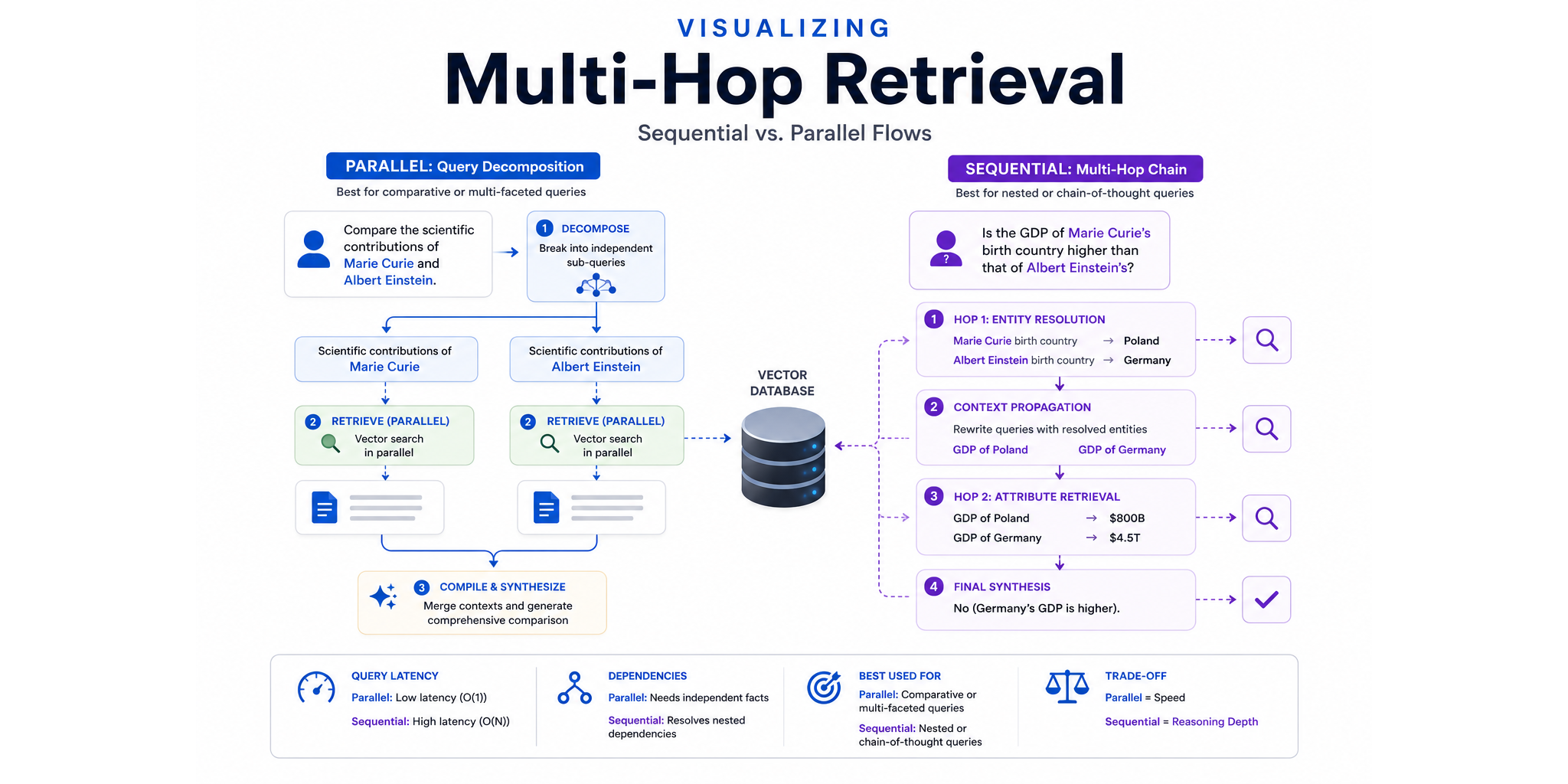
Table of Contents
Introduction
Standard Retrieval-Augmented Generation (RAG) works great for straightforward questions. If you ask for a simple fact, the system searches a vector database, pulls the most relevant document chunk, and uses it to answer.
But what happens when you throw a complex, multi-faceted question at it? Consider this:
"Compare the scientific contributions of Marie Curie and Albert Einstein."
If you pass this entire sentence into a standard RAG pipeline, it creates a single search query. It looks for documents matching the whole phrase, which usually just returns broad biography articles about Curie and Einstein. Because these biographies are generic, they often lack specific details about their scientific breakthroughs, causing the comparison to fail. This is especially true in systems, where we usually set top_k to a small specified value to optimize for speed and cost, making it difficult to retrieve all the necessary information in one go.
Animation 1: Standard RAG retrieves high-level biographies but fails because specific breakthrough details are missing from the retrieved context.
What is Multi-Hop Retrieval?
Multi-hop retrieval solves this problem by breaking a complex query down into multiple, distinct search steps (or "hops"). Instead of executing one broad, cluttered search, the system schedules multiple search steps.
How these searches are scheduled in production typically follows one of two paradigms: Parallel Query Decomposition or Sequential Chains.
Parallel Multi-Hop (Query Decomposition)
If a query is broad and comparative, we can decompose it into independent sub-queries. Since they do not rely on each other's outputs, we can run them at the same time, saving valuable round-trip latency.
For our comparative question:
- Decompilation: The system breaks the main query into independent sub-queries.
- Sub-query 1: "Scientific contributions of Marie Curie"
- Sub-query 2: "Scientific contributions of Albert Einstein"
- Parallel Retrieval: Both sub-queries are launched concurrently against the vector database.
- Executed in parallel to minimize latency, completing in a single round-trip ( latency).
- Compilation: A compiler agent receives the detailed retrieved contexts from both streams and merges them into a clean summary.
Animation 2: Parallel Query Decomposition splits a comparative query into independent sub-queries, running them concurrently to minimize round-trip latency.
Where Query Decomposition Fails
But what happens if we apply query decomposition back to a nested question containing hidden variables? Consider this:
"Is the GDP of Marie Curie's birth country higher than that of Albert Einstein's?"
If a decompiler agent attempts to split this query immediately, it creates two sub-queries: one asking for the GDP of Marie Curie's birth country, and another asking for the GDP of Albert Einstein's birth country.
This hits a wall. The database cannot search for these phrases because GDP documents do not contain the names of scientists, and biography documents do not contain GDP data. The variables [Curie's birth country] and [Einstein's birth country] remain unresolved. We cannot search for a country's GDP until we resolve which country we are looking for.
Animation 3: Immediate decomposition fails on nested queries because it cannot query attributes of unresolved variables.
Sequential Multi-Hop
To solve nested dependencies, we must execute a step-by-step chain of thought. The output of one hop dynamically forms the query for the next.
For our GDP comparison question, sequential retrieval operates in four distinct stages:
- Hop 1 (Entity Resolution): The system first resolves the hidden/unresolved variables by querying biographical details.
- Query 1: "Marie Curie birth country" → returns
Poland - Query 2: "Albert Einstein birth country" → returns
Germany
- Query 1: "Marie Curie birth country" → returns
- Context Propagation: The resolved variables are propagated into the next stage templates.
- Template: "GDP of
[Country 1]" and "GDP of[Country 2]" - Rewritten: "GDP of Poland" and "GDP of Germany"
- Template: "GDP of
- Hop 2 (Attribute Retrieval): The dynamically rewritten queries are executed against the database.
- Query 1: "GDP of Poland" → returns
$800B - Query 2: "GDP of Germany" → returns
$4.5T
- Query 1: "GDP of Poland" → returns
- Final Synthesis: The LLM compiles all step-by-step facts and reasons the final comparison.
- Final Output: "No (Germany's GDP is higher)."
Animation 4: Sequential Multi-Hop resolves nested queries step-by-step, using entity resolution (Hop 1) to propagate variables and rewrite the queries for Hop 2.
Summary of Trade-offs
Choosing the right pattern depends entirely on your data structure and user requirements:
| Feature | Parallel Multi-Hop (Query Decomposition) | Sequential Multi-Hop |
|---|---|---|
| Query Latency | Low ; executes sub-queries concurrently in a single round-trip. | High ; requires sequential database round-trips for each resolved step. |
| Dependencies | Flat / Independent; performs poorly with nested dependencies since it cannot resolve unknown variables. | Nested / Dependent; excels at resolving dependent variables step-by-step. |
| Logic Flow | Static Splitting; simple query splitting without data flow between steps. | Dynamic Propagation; output of a previous hop updates the query template of the next hop. |
| Best Used For | Comparative Queries; comparing multiple entities or attributes simultaneously. | Nested Reasoning; answering questions requiring indirect lookups or attributes of unknown entities. |
Choosing between these flows is a direct trade-off between response speed and reasoning depth. Use parallel query decomposition for flat, comparative queries to keep retrieval times low; use sequential chains for nested, multi-hop reasoning. You can even create a system that combines the parallel query decomposition along with a sequential multi-hop system.